Graph signal processing - application to trafic data analysis

Human societies have always relied on social connection. Today, with the web this is even more true, isn't the internet a huge nebuleous of data ? Networks are also present in our brain, or used to model energy transit.

The goal of this post is to explain how we can interact with graphs supporting one-dimensionnal signals: from data to processing.

^(?)

tl;dr¶

1. Create the adjacency matrix with the appropriate similarity metric.
2. Compute the graph laplacian (from the adjacency matrix) and solve its eigen vectors.
3. Transform the input graph signal into the spectral domain using the laplacian eigen vectors.
4. Enjoy applying any graph convolution on your data!

1. Mathematical background¶

1.1 Graph definition¶

Mathematically, a graph is a pair $G = (V , E)$ where $V$ is the set of vertices, and $E$ are the edges. The vertice or node represent the actual data that is broadcasted through the graph. Each node sends its own signal that propagates through the network. The edges define the relation between these nodes with the weight $w$, the more weighted is the edge, the stronger the relation between two nodes. Some examples of weights can be the vertices distance, signal correlation or even mutual information...

There are many properties for a graph, but the most important one is the directions of the edges. We say that a graph is undirected if for two nodes $a$ and $b$, $w_{ab} = w_{ba}$.

Let's look at the following example which is an unweighted undirected graph (if it was directed we would add arrows instead of lines).

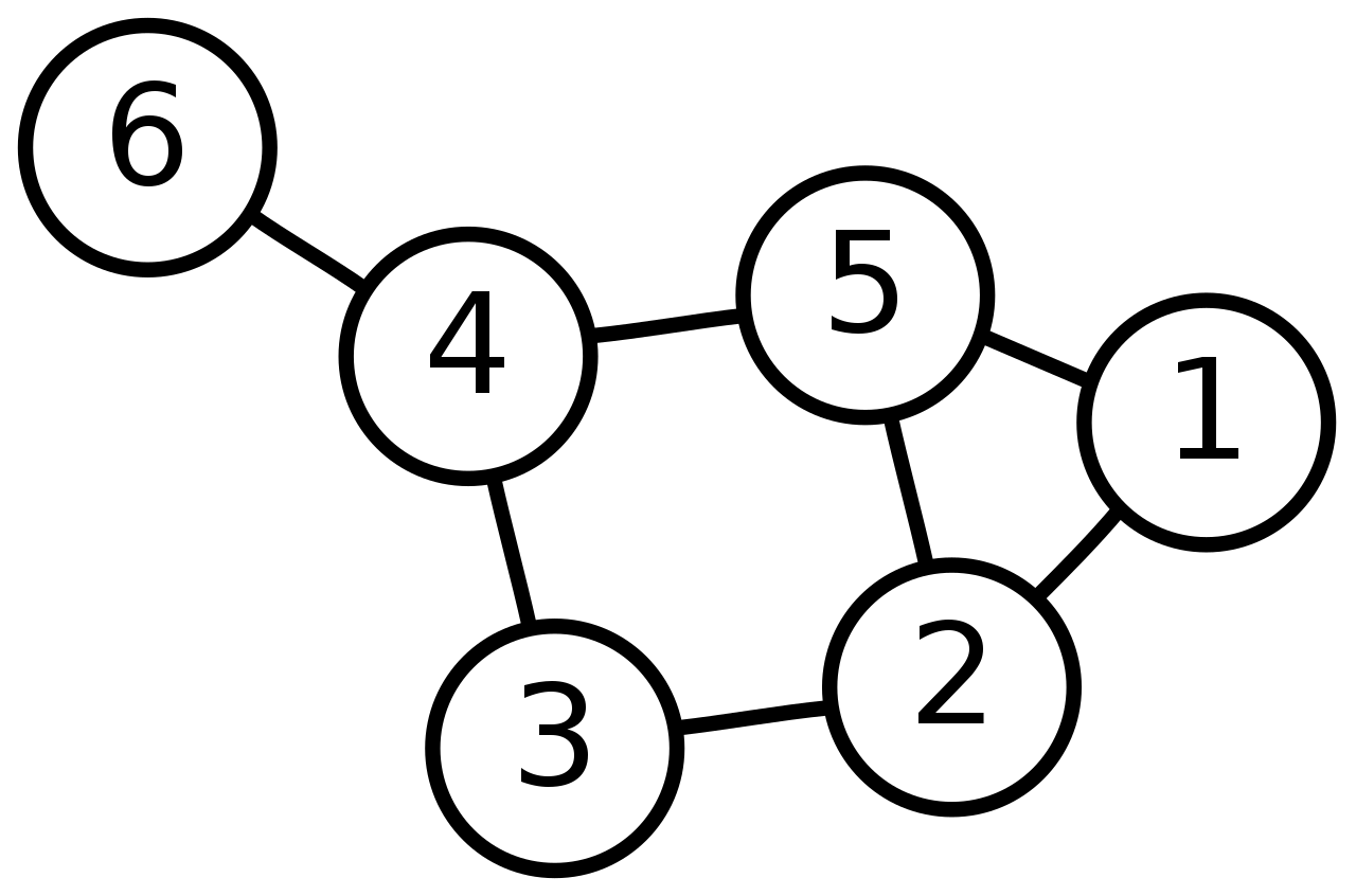
We can use this adjacency matrix $A$ to represent it numerically: \begin{equation} A = \begin{pmatrix} 0 & 1 & 0 & 0 & 1 & 0\\ 1 & 0 & 1 & 0 & 1 & 0\\ 0 & 1 & 0 & 1 & 0 & 0\\ 0 & 0 & 1 & 0 & 1 & 1\\ 1 & 1 & 0 & 1 & 0 & 0\\ 0 & 0 & 0 & 1 & 0 & 0\\ \end{pmatrix} \end{equation}

Each row correspond to the starting node, each column is the ending node. Because it is unweighted, all weights are fixed to $1$, and because it is undirected, the adjecency matrix is symmetric.

In graph signal processing (GSP), the object of study is not the network itself but a signal supported on the vertices of the graph. The graph provides a structure that can be exploited in the data processing. The signal can be any dimension like a single pixel value in an image, images captured by different people or traffic data from radars as we will see after!

If we would assign a random gaussian number for each node of the previous example, the input graph signal $X$ would look like this:

\begin{equation} X = \begin{pmatrix} -1.1875 \\ -0.1841 \\ -1.1499 \\ -1.8298 \\ 1.9561 \\ 0.6322 \end{pmatrix} \end{equation}

For multi-dimensionnal signals (images, volumes), it is common to embed those into a one-dimensionnal latent space to simplify the graph processing. For example if you are working with text features (this could be a tweet from one user, or e-mails), one may use word2vec [1].

1.2 Processing graph signals¶

What we want is to be able to perform operations on those node signals, taking into account the structure of the graph. The most common operation is to filter the signal, or in mathematical term a convolution between a filter $h$ and a function $y$. For example in the temporal domain $t$: \begin{equation} y(t) \circledast h(t) = \int_{-\infty}^{+\infty}{y(t-\tau) h(\tau) d\tau} \end{equation}

Sadly, this is not directly possible in the graph (vertex) domain because the signal translation with $\tau$ is not defined in the context of graphs [2]. How do you perform the convolution then ?

Hopefully, it is much more simple to convolve in the frequency (spectral) domain because we don't need the shift operator. This is also usefull in general in signal processing because it is less intensive computationnally: \begin{equation} \label{fourierconvolution} y(t) \circledast h(t) = Y(\omega) \cdot H(\omega) \end{equation}

To transform the input data (function) into the frequency domain, we use the widely known fourier transform.

It is a reversible, linear transformation that is just the decomposition of a signal into a new basis formed by complex exponentials. The set of complex exponentials are obviously orthogonal (independent) which is a fundamental property to form a basis.

\begin{equation} y(t) \xrightarrow{\mathscr{F}} Y(\omega) = \int_{-\infty}^{\infty} \! y(t) \mathrm{e}^{-i\omega t}\, dt \end{equation}

Note:

In practice, it is not purely reversible because we lose information when applying a fourier transform. Indeed we cannot affoard computationnally to integrate the function over the infinity! We usually use the DFT (Discrete Fourier Transform), which make sense numerically with digital data.

However this formula works in the temporal domain and cannot be applied as is for signal in the graph domain $G$, so how do you define a graph fourier transform ? For that we first need to understand eigen decomposition of the laplacian and its connection to the fourier transform...

1.3 Relation between fourier transform and eigen decomposition¶

The eigen decomposition is a process that is heavily used in data dimension algorithms. For any linear transformation $T$, it exists a non-zero vector (function) $\textbf{v}$ called eigen vector (function) such as:

\begin{equation} \label{eq:eigenfunction} T(\textbf{v}) = \lambda \textbf{v} \end{equation}

Where $\lambda$ is a scalar corresponding to the eigen values, i.e. the importance of each eigen vector. This formula basically means that when we apply the matrix $T$ on $\mathbf{v}$, the resulting vector is co-linear to $\mathbf{v}$. And so $\mathbf{v}$ can be used to define a new orthonormal basis for $T$!

What is of interest for us is that the complex exponential $\mathrm{e}^{i\omega t}$ is also an eigen function for the laplacian operator $\Delta$. Following eq \ref{eq:eigenfunction}, we can derive: \begin{equation} \Delta(e^{i \omega t}) = \frac{\partial^2}{\partial{t^2}} e^{i \omega t} = -\omega^2 e^{i\omega t} \end{equation}

With $\mathbf{v}=e^{i \omega t}$ and eigen values $\lambda = -\omega^2$, which makes sense since we are decomposing the temporal signal into the frequency domain!

We can rewrite the fourier transform $Y(\omega)$ using the conjugate of the eigen function of the laplacian $\mathbf{v}^*$:

\begin{equation} \label{eq:fouriereigen} Y(\omega) = \int_{-\infty}^{\infty} \! y(t) \mathbf{v}^*\,dt \end{equation}

In other word, the expansion of $y$ in term of complex exponential (fourier tranform) is analogeous to the expansion of $y$ in terms of the eigenvectors of the laplacian. Still that does not help on how to apply that to graphs!

1.4 Graph fourier transform¶

There is one specific operation that is well defined for a graph, yes it is the laplacian operator. This is the connection we were looking for and we have now a way to define the graph fourier transform $\mathscr{G}_\mathscr{F}$ !

The graph lalacian $L$ is the second order derivative for a graph, and is simply defined as:

\begin{equation} L = D-A \end{equation}

Where $D$ is the degree matrix that represent the number of nodes connected (including itself).

Intuitively, the graph Laplacian shows in what directions and how smoothly the “energy” will diffuse over a graph if we put some “potential” in node $i$. With the previous example it would be:

\begin{equation} L = \begin{pmatrix} 3 & 0 & 0 & 0 & 0 & 0\\ 0 & 4 & 0 & 0 & 0 & 0\\ 0 & 0 & 3 & 0 & 0 & 0\\ 0 & 0 & 0 & 4 & 0 & 0\\ 0 & 0 & 0 & 0 & 4 & 0\\ 0 & 0 & 0 & 0 & 0 & 2\\ \end{pmatrix} - \begin{pmatrix} 0 & 1 & 0 & 0 & 1 & 0\\ 1 & 0 & 1 & 0 & 1 & 0\\ 0 & 1 & 0 & 1 & 0 & 0\\ 0 & 0 & 1 & 0 & 1 & 1\\ 1 & 1 & 0 & 1 & 0 & 0\\ 0 & 0 & 0 & 1 & 0 & 0\\ \end{pmatrix} \end{equation}

A node that is connected to many other nodes will have a much bigger influence than its neighbours. To mitigate this, it is common to normalize the laplacian matrix using the following formula:

\begin{equation}\label{eq:normlaplacian} L = I - D^{-1/2}AD^{-1/2} \end{equation}

Whith the identity matrix $I$.

After computing the eigen vectors $\mathbf{v}$ for the graph laplacian $L$, we can derive the numeric version of the graph fourier transform $\mathcal{G}$ for $N$ vertices from eq \ref{eq:fouriereigen}:

\begin{equation} \label{eq:graphfouriernumeric} x(i) \xrightarrow{\mathscr{G}_\mathscr{F}} X(\lambda_l) =\sum_{i=0}^{N-1} x(i)\mathbf{v}_l^T(i) \end{equation}

With $x(i)$ being the signal for node $i$ in the graph/vertex domain, which was a single value in our first example.

The matrix form is:

\begin{equation} \label{eq:matrixgraphfouriernumeric} \hat{X} = V^TX \end{equation}

1.5 Global graph convolution¶

Now that we can transform the input data from graph/vertex domain (node $i$) to the spectral domain (frequency $\lambda_l$), we can apply the previous eq \ref{fourierconvolution} to perform graph convolution. We perform the convolution of the data $x$ with filter $h$ into the spectral domain $\lambda_l$, but we want our outputs to be in the graph domain $i$:

\begin{align} x(i) \circledast h(i) & = \mathcal{G}^{-1}(\mathcal{G}(x(i) \circledast h(i))) & \\ & = \sum_{l=0}^{N-1} \hat{x}(\lambda_l) \cdot \hat{g}(\lambda_l) \cdot \mathbf{v}_l^T(i) & \\ \end{align}

and its matrix form [3]:

\begin{align}\label{eq:graphconv} X \circledast H & = V \hat{H} * (V^T X) \end{align}

Warning:

Be carefull of the element wise multiplication in the spectral domain between the filter $\hat{H}$ and transformed data $V^TX$!

One drawback with this method is that is does not work well for dynamic graphs (structure that changes in time) because the eigen vector needs to be recomputed each time! You can also see that this operation is quite complex, hopefully it can be simplified using for example Chebyshev polynomials [4]. The Chebyshev approximation allows to perform local convolution (taking into acount just adjacent nodes) instead of global convolution, which reduces consequently the compute time.

2. Hands on¶

Enough theory, now let's get our hands dirty. We will look into traffic data from the Bay Area and try to analyze it using graph processing.

2.1 Input Data¶

The data that we will be using was originally studied for trafic forecasting in [5]. It consist of a structure with several sensors in the bay area (California) that acquired the speed of cars (in miles/hour) during 6 months of year 2017. It is available publically and was collected by California Transportation Agencies Performance Measurement System (PeMS).

There are two files, sensor_locations_bay_area.csv consists of the locations of each sensor (that can be used to define the structure of the graph), the other file traffic_bay_area.csv includes the drivers speed gathered by each sensor (the node feature).

All the sensors are located in the Bay Area of San francisco, as you can see with the following map.

2.2 Graph construction¶

The most important step when constructing a graph is how to define the relationships between nodes. Mathematically, we craft a positive metric bounded between $[0, 1]$ that should be high when the relation between those two nodes is strong, and as much linear as possible. Then we can model the graph using the adjacency matrix, where each line/column index being one node ID.

Here we use the euclidean distance between nodes as a metric (the distance matrix $D$). To simplify this post, we will suppose a weighted undirected graph (which in practice is maybe not ideal since cars go in one direction).

2.2.1 Adjacency matrix¶

Let's first try to build the adjacency matrix using the sensor locations. We will compute the euclidean distance between each sensor to define the realtionship between nodes.

We are working with geodesic position which lives on a sphere, hence it is not advised to directly use those positions to compute the euclidean distances. First, we need to project those into a plane, following the assumption that the measurements are close to each other, one can use the equirectangular projection.

Now we can compute the distances.

We craft the adjacency matrix $A$ by inverting and normalizing the current distance matrix $D$, so the edge weights are high when the relation is high (nodes are spatially closed). The resulting distance matrix is symmetric, with the number of rows/columns equal to the number of sensors.

2.2.2 Pre-processing the graph¶

Because we have lot of nodes (325 sensors), the resulting graph is huge with more than $325\times325>1e^7$ edges! Using a graph that has lot of edges is not practical in our case, as this would require more CPU power with high RAM usage, hence we need to downsample the graph.

The topic of downsampling or pre-processing spatiotemporal graph is itself really active [6], here we use a simple thresholded approach called nearest neighbor graph (k-nn): keep the $k$ most important neighbor (for each node). This prevents orphan nodes compare to a basic thresholding approach.

Another additionnal process is removing the so-called "self-loops" (i.e. make the diagonal zero), so nodes does not have a relation with themself.

Looking at the adjacency matrix itself, it is now much cleaner. We see that the adjacency matrix is really sparse, this is because sensors indexes does not have spatial meaning (sensor $i=0$ and $i=1$ can be far away).

But is it logical to just use the distance matrix as a metric? What happens if there are sensors that are spatially really close, but not on the same lane?

Take for example two sensors #400296 and #401014 (near the highway interchange California 237/Zanker road on the map) and let's look at their traffic measurements on Monday 3 Apr 2017.

Those are really uncorrelated, whereas the more distant sensors #400296 and #400873 are much more correlated (because they are on the same direction lane).

To take into account this, we use the correlation matrix to filter out "bad" edges. We compute the correlation just for a single day (to mitigate seasonal effects), and every edges that have a correlation less than $0.6$ will be disgarded.

2.2.3 Analyzis and visualization¶

To plot the graph, we installed the networkx package [7], you can find the documentation here.

This graph mainly follows the structure of the main roads in the bay area, because this is where the sensors are. Still, it also features some interconnections mostly due to the inner road connexions of the city.

2.3 Spectral decomposition¶

Now that we defined the graph structure, we can start the spectral decomposition. We will need that to perform the graph convolution, and there are also interresting visualization to better understand the graph structure.

2.3.1 Normalized laplacian matrix¶

As a reminder, we apply the eq \ref{eq:normlaplacian} using the degree matrix and the adjacency matrix.

2.3.2 Eigen decomposition¶

After the laplacian is defined, we can now eigen decompose the matrix. Because our matrix is real and symmetric, we can use np.linalg.eigh which is faster than the original np.linalg.eig.

An important thing to check is if the eigen vectors carries a notion of frequency, for a graph that is simply the number of time each eigen vector change sign, or number of zero-crossings [8].

Minus the noise, the tendency is that the larger the eigen values $\lambda_l$, the higher the frequency (more zero-crossings between nodes). Also all the eigen values are positive, that would not be the case if the laplacian matrix was not symmetric.

We can also try to interpret what the eigen vectors are responsible for, by projecting it on the graph (similar to what we would do to analyse deep learning filters). In the figure below, it is clear that an eigen vector with higher eigen value leads to a higher frequency graph.

Some clear patterns can be distinguished, for example eigen vector #1 seems to be responsible for eastern sensors.

2.4 Clustering¶

It is relatively easy to apply clustering, even with unlabelled data. What you want to do is perform a simple unsupervised clustering (like k-means) on the lowest eigen vectors. Why on the low frequencies? Because they carry the power of the signal, when the highest frequency carry the dynamic of the graph. Here we will try to use the first $5$ eigen vectors.

This result in the clustering of some western sensors, interrestingly it does not cluster all the sensors on the same road, but just those who are on the same lane/direction. This is because of the constrain that we put on the graph, taking into acount correlation of the data!

2.5 Filtering¶

We saw in the mathematical background section that we can easily filter a signal in the spectral domain, let's implement this using eq \ref{eq:graphconv}.

In classical signal processing, a filter can be easilly translated into the temporal domain. This is not possible in GSP (translate a filter into the graph domain), however it is possible to check its response in our system by convolving the filter with a dirac. Let's try to apply a heat filter on our graph and see its response in the vertex domain.

Here is the result when applying the heat filter to $\delta_{0}$ (at the position of the node #400001 located at the interchange US 101/Miami 880).

This can help us interprate how the energy diffuse over the system, for this specific example it can be a tool for engineers to see where traffic congestion can happen. Good luck for the drivers in the center of bay area!

Applying this filter to the sensor measurements acts a (really) low pass filter, as you can see below.

Why is the resulting signal lower? I suppose this is because the offset component is partially canceled out after filtering (in our case the minimum frequency is not zero but $\lambda_0 = 0.048$).

Conclusion¶

This post guided you on how the graph signal processing theory was built, and how to apply it concretely. We saw a specific example using traffic data, and although we could go much further in the analysis, I hope it answered some of your questions

To go gurther¶

A first reference that helped me a lot for my understanding is the Stanford class CS224W: Machine Learning with Graphs. Also the Persagen Consulting web page which are specialized in molecular genetics, but still is a really good ressource.

The extension of GSP applied to deep learning is the hot topic of graph convolution networks (GCN). If you are curious about them definitively look at this wonderfull distill interactive post. Also, I was lucky to work with Dr Zhang specifically on applying GCNs to neuroimaging data (fMRI), check her work!

Finally, the set of tutorials from pygsp are also a great way to understand each component of GSP.

References ¶

References

1. Mikolov, T., Chen, K., Corrado, G., Dean, J.: Efficient estimation of word representations in vector space. arXiv preprint arXiv:1301.3781. (2013).
2. Nonato, L.G.: Graph Fourier Transform, (2017). https://doi.org/https://sites.icmc.usp.br/gnonato/gs/slide3.pdf.
3. Kipf, T.N., Welling, M.: Semi-supervised classification with graph convolutional networks. arXiv preprint arXiv:1609.02907. (2016).
4. Hammond, D.K., Vandergheynst, P., Gribonval, R.: Wavelets on graphs via spectral graph theory. Applied and Computational Harmonic Analysis. 30, 129–150 (2011).
5. Li, Y., Yu, R., Shahabi, C., Liu, Y.: Diffusion convolutional recurrent neural network: Data-driven traffic forecasting. arXiv preprint arXiv:1707.01926. (2017).
6. Leskovec, J., Faloutsos, C.: Sampling from large graphs. In: Proceedings of the 12th ACM SIGKDD international conference on Knowledge discovery and data mining. pp. 631–636 (2006).
7. Hagberg, A.A., Schult, D.A., Swart, P.J.: Exploring Network Structure, Dynamics, and Function using NetworkX. In: Varoquaux, G., Vaught, T., and Millman, J. (eds.) Proceedings of the 7th Python in Science Conference. pp. 11–15. , Pasadena, CA USA (2008).
8. Shuman, D.I., Narang, S.K., Frossard, P., Ortega, A., Vandergheynst, P.: The emerging field of signal processing on graphs: Extending high-dimensional data analysis to networks and other irregular domains. IEEE signal processing magazine. 30, 83–98 (2013).